Building a RAG Pipeline for Semantic Code Search: A Developer Diary and Field Notes

以下正文同步自 JetBrains Blog，版权归原站所有，已转换为易读排版。

Part 1: Parsing, chunking, and vectorization

Some time ago, we set out to build the best semantic code search platform we could: a RAG pipeline that gives LLM agents precise, citable evidence from real repositories instead of whatever grep happens to surface. The eventual solution was JetBrains Context. We got it working, we got it into production, and we collected a lot of scar tissue along the way. In this series of posts, we’ll share the parts we wish someone had told us on day one.

Coding agents are undoubtedly the biggest technology leap for software development of our decade. Agents and frontier models are proving their aptitude in the face of seemingly insurmountable code complexity to produce ostensibly reliable code.

However, as more and more development processes become agent-driven, the agent’s efficiency and the quality of the produced code become increasingly important. The question is not so much about whether an agent can complete the task, as given enough time and token resources, it surely will, but rather how much time, effort, and steering is required for it to generate production-grade results. For large-scale code bases specifically, the agent would spend a great deal of time searching for the relevant pieces of code relevant for the feature it’s working on and pulling them into the context.

Why semantic search matters

Attempting to locate the right code snippets, the agent will resort to traditional tools for code search such as keyword search and grep. These tools, however, are limited in that they require the agent to know in advance which exact text to search for. For example, an agent looking for where session tokens get refreshed cannot rely on the code helpfully containing the word “refresh”. To reason through abstract domains, the agent needs the ability to search for code by meaning, also known as semantic search. This is where retrieval-augmented generation (RAG) comes into the picture. If we can index the source code in a way that captures its semantics and then allow the agent to retrieve the relevant pieces on demand using free text search, we create an interface that plays to the agent’s strengths.

From prototype to production

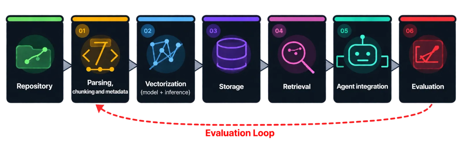
Like many great ideas in the agentic era, a native, prototype implementation is extremely simple. A well-evaluated production grade solution most certainly is not. In this series of blog posts, we want to share what is involved in making an effective RAG system, as well as the wrong turns we took in our journey to create our own: JetBrains Context. We’ll tackle each stage, from pre-processing to storage and agent integration, providing some more technical context and advice.

This first part of the series will cover the initial stages of the pipeline: parsing and chunking, where raw source files are divided into properly scoped units, and vectorization, where those units are transformed into a representation that supports semantic search.

The fine AST of parsing and chunking

Parsing and chunking is a critical pre-processing step in a good RAG solution, but it is often overlooked. In order to allow the LLM to embed or otherwise index the source code, we must first feed it the raw lines of code. This may sound trivial, and probably would be for small-scale demo projects. However, production-grade systems contain thousands of files, which, in turn, span hundreds or even thousands of lines. If anything, agents have compounded the problem, as they tend to be prolific writers, further inflating the codebase. Each file may contain multitudes of classes, fields, and methods, with varying degrees of relatedness among them.

Finding the right chunk size

Even if it were possible to fit these huge code files into an embedding model in their entirety, that expensive feat would ultimately be self-defeating. Because the entire file was embedded in a single unit, the search would return the entire file. This is counterproductive to the goals of agentic code exploration and navigation, which are mostly concerned with finding a specific function, symbol, or code snippet.

On the other hand, if we were to take the other extreme and granularly embed each separate line of code, we would be facing a problem of a different sort. These individual lines can be semantically insignificant without the surrounding context. A generic function name or comment does not merit embedding and will produce the wrong retrieval result. In a sense, we would not be able to see the forest for the trees, and the agent would be overloaded with multiple, often insignificant micro-results.

It is therefore imperative to find the right method to chunk or divide the code into groups that are properly scoped. Each group should include enough of the necessary context and represent common semantic meaning.

Why fixed-size chunking falls short

Chunking is a generic name for the technique of taking content that will be fed to the agent and dividing it into a set of chunks. A naive approach to chunking could be simply splitting a large file into groups with a fixed number of lines. However, if we were to take that approach, we would find the resulting groupings semantically wrong. Unrelated code pieces would be grouped together, for example, an import statement and some function content, leading to mistakes during retrieval.

To solve the problem, we can leverage the fact that every source file has a pretty well-defined structure. Take Java as an example – imports tend to be at the top of the file, followed by a class definition with an optional doc-comment preceding the header. The class will contain fields and methods, which in turn may also have their own doc-comments. Knowing about the conventions and rules that define the class structure allows us to perform smarter chunking and achieve the right balance of surrounding information.

Parsing and structure-aware chunking

Over the last 26 years, we at JetBrains have developed parsers that are smart enough to adjust for the various quirks, irregularities, conventions, and nuances of specific languages. Alongside other tools, these parsers form our internal JetBrains Code Engine platform on which JetBrains Context is developed. At the moment of this article’s composition, JetBrains Context supports parsing and structure-aware chunking for nine major languages: Kotlin, Java, Python, JavaScript, TypeScript, C#, PHP, Go, and Rust. For all other languages, our implementation simply falls back to naive, line-based splitting to ensure that any language or document can be indexed and searched.

The parser allows us to break source files into streams of syntax nodes that carry information about what they represent – comments, whitespaces, lists of modifiers, and so on. The chunking algorithm then consumes that stream and applies logic that decides the scope of a given chunk. Based on the node’s type and size, as well as its descendants, the algorithm makes a decision. If a node exceeds the size threshold but has no children, it will fall back to more primitive splitting strategies.

Some language-specific constructs are kept as single slices even if they exceed the preferred size. Prefixes such as documentation, annotations, visibility modifiers, and keywords are kept together with the declaration; suffixes (usually closing syntax) remain associated with the construct they close. There is also some language-specific cleaning, where, for instance, common and semantically meaningless Java annotations such as @NotNull or @Override are removed.

The algorithm bears some similarities to cAST, authored by Zhang et al. in 2025. Both our implementation and cAST retain the largest syntax units that fit, subdividing only the units that are too large, and grouping smaller adjacent units to avoid tiny chunks that are not usually semantically meaningful. The biggest difference is that we coded more language semantics into our implementation, keeping Python decorators together with definitions, KDocs next to Kotlin declarations, and so on.

After grouping, chunk normalization is performed, which involves:

- Trimming leading and trailing whitespaces

- Deleting blank lines

- Removing common indentation while preserving relative indentation

Following the normalization procedure, the chunk is then passed to the next step – embedding – along with metadata that consists of a relative path, which gets embedded alongside the normalized chunk content.

Evaluating the quality of chunks

It is hard to give a concrete answer as to what the input to the embedding model should look like. Chunk size matters, but as discussed before, bigger is not always better. Additionally, some metadata embedded alongside the code may be useful, while some may introduce noise that ultimately decreases search quality.

We opted to use an LLM-as-a-judge strategy to inspect the chunks as a part of the evaluation. The judge, using a chunk and the source file, considers whether the boundary makes sense. It looks for unexpected artifacts, such as detached documentation, orphaned closing syntax, or fragments of code that are cut through a meaningful construct. In addition, any changes to the source code processing pipelines also go through the full, end-to-end retrieval evaluation. We’ll get back to that evaluation pipeline in the following part of this series.

Vectorization

Having pre-processed the source code, we finally have text chunks that are hopefully just the right size and correctly grouped for semantic retrieval. Our next task is to transform these fragments in a way that will later allow us to support semantic search, through a process called vectorization.

With vectorization, an embedding model reads a piece of text and emits a fixed-length list of numbers (a vector), which amounts to a point in a space of a few thousand dimensions. Significantly, the model is trained so that texts with similar meaning land close together. Traditional search might miss the connection, but here, a function that flushes buffered write operations and one that drains a pending queue can end up near each other despite sharing no common keywords. The distance between vectors hence becomes a measure of relatedness. A query is turned into a position in the same space, and the results are whatever lies nearest to it.

Punch for the byte: Optimizing for storage

Any attempt to vectorize a large codebase must take into account both cost and performance. A single embedding is cheap, but a large repository produces millions of chunks, which become millions of vectors that must be stored, held in memory, and compared against each incoming query. A vector of a few thousand dimensions in 32-bit floats weighs around 16 kilobytes, so a few million chunks add up to tens of gigabytes of index before any bookkeeping. At such a scale, the allocation of bytes per vector becomes cost-limited, and the leading question quickly shifts from “how accurate can we be?” to “what do we get per byte?” In other words, we need to find a way to reduce the cost while retaining as much search quality as possible.

There are two ways to reduce vector cost. The first is to keep fewer dimensions. Modern embedding models are trained so that a leading slice of the vector works on its own. The dimension loss is applied across several nested prefix lengths simultaneously, pushing the coarsest structure into the earliest dimensions. This means you can cut a vector short and renormalize it, and it still retrieves. Alternatively, you can keep every dimension and spend less on each one by sacrificing on precision and thus keeping fewer bytes for each vector.

These two options are independent of each other and can be combined, which means any storage budget can be met through different mixes of dimension count and numeric precision. The real question is which mix retrieves best for the same number of bytes. The trade-off is far from even. Suppose the budget is 512 bytes per vector. You could spend it on 128 dimensions kept at full 32-bit precisi

正文由 FLUX 从来源站点 RSS 同步，内容未经改写；遇到排版缺失或需要图片、视频时请以原文为准。